idrlnet/docs/user/get_started/1_simple_poisson.md

# Solving Simple Poisson Equation

Inspired by [Nvidia SimNet](https://developer.nvidia.com/simnet), 
IDRLnet employs symbolic links to construct a computational graph automatically.
In this section, we introduce the primary usage of IDRLnet.
To solve PINN via IDRLnet, we divide the procedure into several parts:

1. Define symbols and parameters.
1. Define geometry objects.
1. Define sampling domains and corresponding constraints.
1. Define neural networks and PDEs.
1. Define solver and solve.
1. Post processing.

We provide the following example to illustrate the primary usages and features of IDRLnet.

Consider the 2d Poisson's equation defined on $\Omega=[-1,1]\times[-1,1]$, which satisfies $-\Delta u=1$, with
the boundary value conditions:

$$
\begin{align}
\frac{\partial u(x, -1)}{\partial n}&=\frac{\partial u(x, 1)}{\partial n}=0 \\
u(-1,y)&=u(1, y)=0
\end{align}
$$

## Define Symbols
For the 2d problem, we define two coordinate symbols `x` and `y`, which will be used in symbolic expressions in IDRLnet.
```python
x, y = sp.symbols('x y')
```
Note that variables `x`, `y`, `z`, `t` are reserved inside IDRLnet. 
The four symbols should only represent the 4 primary coordinates.

## Define Geometric Objects

The geometry object is a simple rectangle.
```python
rec = sc.Rectangle((-1., -1.), (1., 1.))
```

Users can sample points on these geometry objects. The operators `+`, `-`, `&` are also supported. 
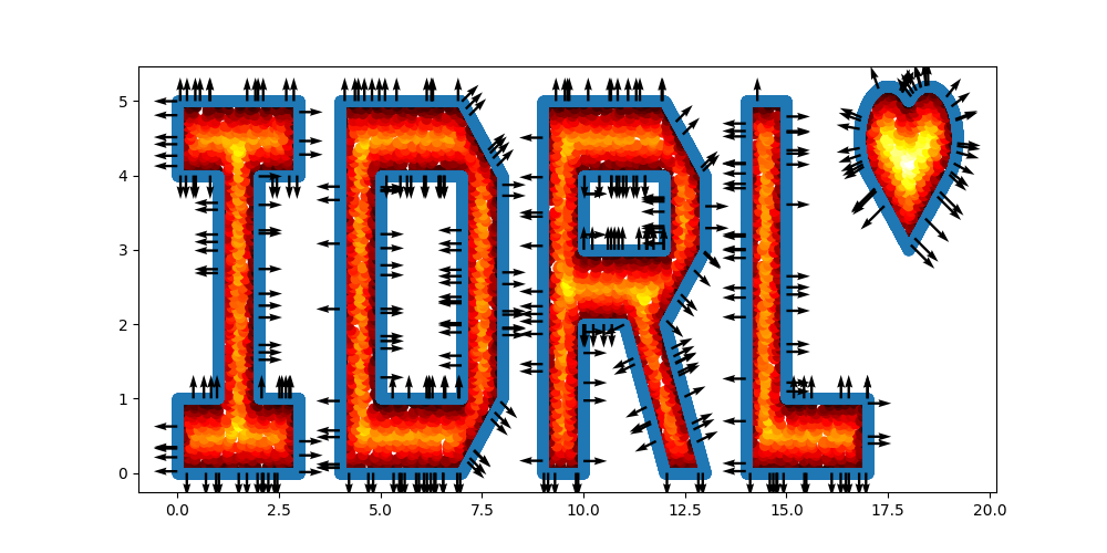
A slightly more complicated example is as follows:
```python
import numpy as np
import idrlnet.shortcut as sc

# Define 4 polygons
I = sc.Polygon([(0, 0), (3, 0), (3, 1), (2, 1), (2, 4), (3, 4), (3, 5), (0, 5), (0, 4), (1, 4), (1, 1), (0, 1)])
D = sc.Polygon([(4, 0), (7, 0), (8, 1), (8, 4), (7, 5), (4, 5)]) - sc.Polygon(([5, 1], [7, 1], [7, 4], [5, 4]))
R = sc.Polygon([(9, 0), (10, 0), (10, 2), (11, 2), (12, 0), (13, 0), (12, 2), (13, 3), (13, 4), (12, 5), (9, 5)]) \
    - sc.Rectangle(point_1=(10., 3.), point_2=(12, 4))
L = sc.Polygon([(14, 0), (17, 0), (17, 1), (15, 1), (15, 5), (14, 5)])

# Define a heart shape.
heart = sc.Heart((18, 4), radius=1)

# Union of the 5 geometry objects
geo = (I + D + R + L + heart)

# interior samples
points = geo.sample_interior(density=100, low_discrepancy=True)
plt.figure(figsize=(10, 5))
plt.scatter(x=points['x'], y=points['y'], c=points['sdf'], cmap='hot')

# boundary samples
points = geo.sample_boundary(density=400, low_discrepancy=True)
plt.scatter(x=points['x'], y=points['y'])
idx = np.random.choice(points['x'].shape[0], 400, replace=False)

# Show normal directions on boundary
plt.quiver(points['x'][idx], points['y'][idx], points['normal_x'][idx], points['normal_y'][idx])
plt.show()
```
![Geometry](https://raw.githubusercontent.com/weipeng0098/picture/master/20210617081809.png)

## Define Sampling Methods and Constraints
Take a 1D fitting task as an example.
The data source generates pairs $(x_i, f_i)$. We train a network $u_\theta(x_i)\approx f_i$.
Then $f_i$ is the target output of $u_\theta(x_i)$. 
These targets are called constraints in IDRLnet.

For the problem, three constraints are presented.

The constraint

$$
u(-1,y)=u(1, y)=0
$$
is translated into
```python
@sc.datanode
class LeftRight(sc.SampleDomain):
    # Due to `name` is not specified, LeftRight will be the name of datanode automatically
    def sampling(self, *args, **kwargs):
        # sieve define rules to filter points
        points = rec.sample_boundary(1000, sieve=((y > -1.) & (y < 1.)))
        constraints = sc.Variables({'T': 0.})
        return points, constraints
```
Then `LeftRight()` is wrapped as an instance of `DataNode`. 
One can store states in these instances.
Alternatively, if users do not need storing states, the code above is equivalent to
```python
@sc.datanode(name='LeftRight')
def leftright(self, *args, **kwargs):
    points = rec.sample_boundary(1000, sieve=((y > -1.) & (y < 1.)))
    constraints = sc.Variables({'T': 0.})
    return points, constraints
```
Then `sampling()` is wrapped as an instance of `DataNode`. 

The constraint

$$
\frac{\partial u(x, -1)}{\partial n}=\frac{\partial u(x, 1)}{\partial n}=0
$$
is translated into

```python
@sc.datanode(name="up_down")
class UpDownBoundaryDomain(sc.SampleDomain):
    def sampling(self, *args, **kwargs):
        points = rec.sample_boundary(1000, sieve=((x > -1.) & (x < 1.)))
        constraints = sc.Variables({'normal_gradient_T': 0.})
        return points, constraints
```
The constraint `normal_gradient_T` will also be one of the output of computable nodes, including `PdeNode` or `NetNode`.

The last constraint is the PDE itself $-\Delta u=1$:

```python
@sc.datanode(name="heat_domain")
class HeatDomain(sc.SampleDomain):
    def __init__(self):
        self.points = 1000

    def sampling(self, *args, **kwargs):
        points = rec.sample_interior(self.points)
        constraints = sc.Variables({'diffusion_T': 1.})
        return points, constraints
```
`diffusion_T` will also be one of the outputs of computable nodes. 
`self.points` is a stored state and can be varied to control the sampling behaviors.

## Define Neural Networks and PDEs
As mentioned before, neural networks and PDE expressions are encapsulated as `Node` too.
The `Node` objects have `inputs`, `derivatives`, `outputs` properties and the `evaluate()` method.
According to their inputs, derivatives, and outputs, these nodes will be automatically connected as a computational graph.
A topological sort will be applied to the graph to decide the computation order.

```python
net = sc.get_net_node(inputs=('x', 'y',), outputs=('T',), name='net1', arch=sc.Arch.mlp)
```
This is a simple call to get a neural network with the predefined architecture.
As an alternative, one can specify the configurations via
```python
evaluate = MLP(n_seq=[2, 20, 20, 20, 20, 1)], 
                activation=Activation.swish, 
                initialization=Initializer.kaiming_uniform,
                weight_norm=True)
net = NetNode(inputs=('x', 'y',), outputs=('T',), net=evaluate, name='net1', *args, **kwargs)
```
which generates a node with
- `inputs=('x','y')`, 
- `derivatives=tuple()`, 
- `outpus=('T')`
```python
pde = sc.DiffusionNode(T='T', D=1., Q=0., dim=2, time=False)
```
generates a node with
- `inputs=tuple()`, 
- `derivatives=('T__x', 'T__y')`, 
- `outputs=('diffusion_T',)`.

```python
grad = sc.NormalGradient('T', dim=2, time=False)
```
generates a node with
- `inputs=('normal_x', 'normal_y')`, 
- `derivatives=('T__x', 'T__y')`, 
- `outputs=('normal_gradient_T',)`.
The string `__` is reserved to represent the derivative operator. 
If the required derivatives cannot be directly obtained from outputs of other nodes,
It will try `autograd` provided by Pytorch with the maximum prefix match from outputs of other nodes.

## Define A Solver
Initialize a solver to bundle all the components and solve the model.
```python
s = sc.Solver(sample_domains=(HeatDomain(), LeftRight(), UpDownBoundaryDomain()),
              netnodes=[net],
              pdes=[pde, grad],
              max_iter=1000)
s.solve()
```
Before the solver start running, it constructs computational graphs and applies a topological sort to decide the evaluation order. 
Each sample domain has its independent graph.
The procedures will be executed automatically when the solver detects potential changes in graphs.
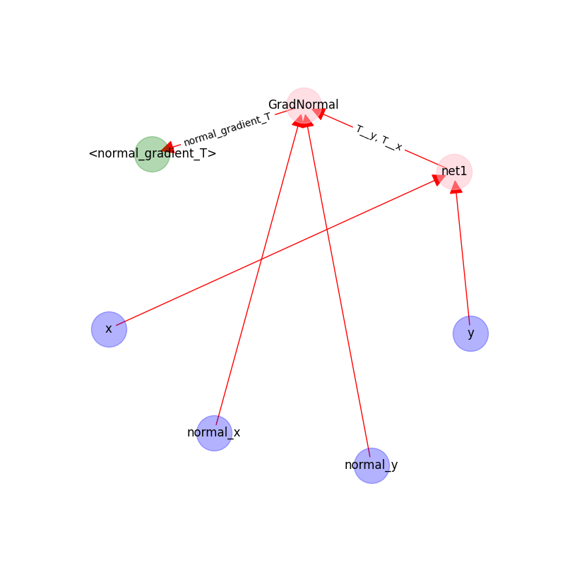
As default, these graphs are also visualized as `png` in the `network` directory named after the corresponding domain.

The following figure shows the graph on `UpDownBoundaryDomain`:
![up_down](https://raw.githubusercontent.com/weipeng0098/picture/master/20210617081822.png)

- The blue nodes are generated via sampling; 
- the red nodes are computational; 
- the green nodes are constraints(targets).

## Inference
We use domain `heat_domain` for inference. 
First, we increase the density to 10000 via changing the attributes of the domain.
Then, `Solver.infer_step()` is called for inference.
```python
s.set_domain_parameter('heat_domain', {'points': 10000})
coord = s.infer_step({'heat_domain': ['x', 'y', 'T']})
num_x = coord['heat_domain']['x'].cpu().detach().numpy().ravel()
num_y = coord['heat_domain']['y'].cpu().detach().numpy().ravel()
num_Tp = coord['heat_domain']['T'].cpu().detach().numpy().ravel()
```

One may also define a separate domain for inference, which generates `constraints={}`, and thus, no computational graphs will be generated on the domain.
We will see this later. 

## Performance Issues
1. When a domain is contained by `Solver.sample_domains`, the `sampling()` will be called every iteration.
   Users should avoid including redundant domains. 
   Future versions will ignore domains with `constraints={}` in training steps.
2. The current version samples points in memory. 
   When GPU devices are enabled, data exchange between the memory and GPU devices might hinder the performance.
   In future versions, we will sample points directly in GPU devices if available.
   
See `examples/simple_poisson`.