forked from idrl/idrlnet
110 lines
4.3 KiB
Markdown
110 lines
4.3 KiB
Markdown
|
|
# Allen-Cahn Equation
|
||
|
|
|
||
|
|
This section repeats the adaptive PINN method presented by [Wight and Zhao][1].
|
||
|
|
|
||
|
|
The Allen-Cahn equation has the following general form:
|
||
|
|
|
||
|
|
$$ \partial_{t} u=\gamma_{1} \Delta u+\gamma_{2}\left(u-u^{3}\right). $$
|
||
|
|
|
||
|
|
Consider the one-dimensional Allen-Cahn equation with periodic boundary conditions:
|
||
|
|
|
||
|
|
$$
|
||
|
|
\begin{array}{l}
|
||
|
|
u_{t}-0.0001 u_{x x}+5 u^{3}-5 u=0, \quad x \in[-1,1], \quad t \in[0,1], \\
|
||
|
|
u(0, x)=x^{2} \cos (\pi x) \\
|
||
|
|
u(t,-1)=u(t, 1) \\
|
||
|
|
u_{x}(t,-1)=u_{x}(t, 1).
|
||
|
|
\end{array}
|
||
|
|
$$
|
||
|
|
|
||
|
|
## Periodic Boundary Conditions
|
||
|
|
|
||
|
|
The periodic boundary conditions are enforced by $u(t, x)=u(t,x+2)$ and $u_x(t, x)=u_x(t,x+2)$ with $x=-1$, which is
|
||
|
|
equivalent to
|
||
|
|
|
||
|
|
$$
|
||
|
|
\begin{array}{l}
|
||
|
|
\tilde u(t,x)=u(t,x+2), \quad \forall t\in[0,1],x\in[-1,1], \\
|
||
|
|
\tilde u(t,x)=u(t,x),\quad \forall t\in[0,1],x=-1, \\
|
||
|
|
\tilde u_x(t,x)=u_x(t,x),\quad \forall t\in[0,1],x=-1.\\
|
||
|
|
\end{array}
|
||
|
|
$$
|
||
|
|
|
||
|
|
The transform above is implemented by
|
||
|
|
|
||
|
|
```python
|
||
|
|
net_u = sc.MLP([2, 128, 128, 128, 128, 2], activation=sc.Activation.tanh)
|
||
|
|
net_u = sc.NetNode(inputs=('x', 't',), outputs=('u',), name='net1', net=net_u)
|
||
|
|
xp = sc.ExpressionNode(name='xp', expression=x + 2)
|
||
|
|
net_tilde_u = sc.get_shared_net_node(net_u, inputs=('xp', 't',), outputs=('up',), name='net2', arch='mlp')
|
||
|
|
```
|
||
|
|
|
||
|
|
where `xp` translates $x$ to $x+2$. The node `net_tilde_u` has the same internal parameters as `net_u` while its inputs
|
||
|
|
and outputs are translated.
|
||
|
|
|
||
|
|
## Receivers acting as Callbacks
|
||
|
|
We define a group of `Signal` to trigger receivers.
|
||
|
|
They are adequate for customizing various PINN algorithms at the moment.
|
||
|
|
|
||
|
|
```python
|
||
|
|
class Signal(Enum):
|
||
|
|
REGISTER = 'signal_register'
|
||
|
|
SOLVE_START = 'signal_solve_start'
|
||
|
|
TRAIN_PIPE_START = 'signal_train_pipe_start'
|
||
|
|
AFTER_COMPUTE_LOSS = 'compute_loss'
|
||
|
|
BEFORE_BACKWARD = 'signal_before_backward'
|
||
|
|
TRAIN_PIPE_END = 'signal_train_pipe_end'
|
||
|
|
SOLVE_END = 'signal_solve_end'
|
||
|
|
```
|
||
|
|
|
||
|
|
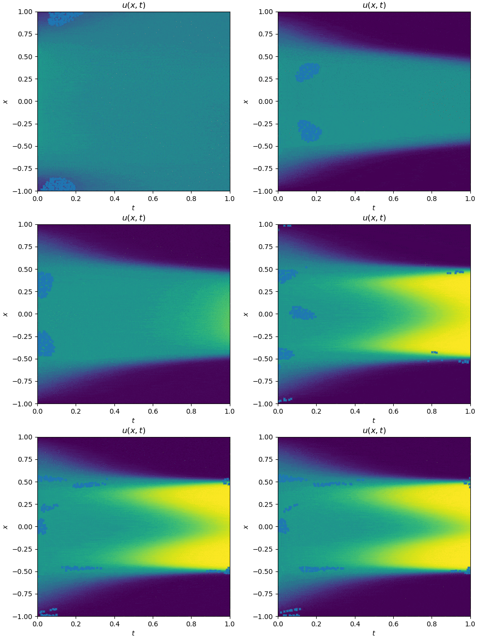
We implement the adaptive sampling method as follows.
|
||
|
|
```python
|
||
|
|
class SpaceAdaptiveReceiver(sc.Receiver):
|
||
|
|
# implement the abstract method in sc.Receiver
|
||
|
|
def receive_notify(self, solver, message):
|
||
|
|
# In each iteration, after the train pipe ends, the receiver will be notified.
|
||
|
|
# Every five 500 iterations, the adaptive sampling will be triggerd.
|
||
|
|
if sc.Signal.TRAIN_PIPE_END in message.keys() and solver.global_step % 1000 == 0:
|
||
|
|
sc.logger.info('space adaptive sampling...')
|
||
|
|
# Do extra sampling and compute the residual
|
||
|
|
results = solver.infer_step({'data_evaluate': ['x', 't', 'sdf', 'AllenCahn_u']})
|
||
|
|
residual_data = results['data_evaluate']['AllenCahn_u'].detach().cpu().numpy().ravel()
|
||
|
|
# Sort the points by residual loss
|
||
|
|
index = np.argsort(-1. * np.abs(residual_data))[:200]
|
||
|
|
_points = {key: values[index].detach().cpu().numpy() for key, values in results['data_evaluate'].items()}
|
||
|
|
_points.pop('AllenCahn_u')
|
||
|
|
_points['area'] = np.zeros_like(_points['sdf']) + (1.0 / 200)
|
||
|
|
# Update the points in the re_samping_domain
|
||
|
|
solver.set_domain_parameter('re_sampling_domain', {'points': _points})
|
||
|
|
```
|
||
|
|
We also draw the result every $1000$ iterations.
|
||
|
|
```python
|
||
|
|
class PostProcessReceiver(Receiver):
|
||
|
|
def receive_notify(self, solver, message):
|
||
|
|
if pinnnet.receivers.Signal.TRAIN_PIPE_END in message.keys() and solver.global_step % 1000 == 1:
|
||
|
|
points = s.infer_step({'allen_test': ['x', 't', 'u']})
|
||
|
|
triang_total = tri.Triangulation(points['allen_test']['t'].detach().cpu().numpy().ravel(),
|
||
|
|
points['allen_test']['x'].detach().cpu().numpy().ravel(), )
|
||
|
|
plt.tricontourf(triang_total, points['allen_test']['u'].detach().cpu().numpy().ravel(), 100)
|
||
|
|
tc_bar = plt.colorbar()
|
||
|
|
tc_bar.ax.tick_params(labelsize=12)
|
||
|
|
plt.xlabel('$t$')
|
||
|
|
plt.ylabel('$x$')
|
||
|
|
plt.title('$u(x,t)$')
|
||
|
|
plt.savefig(f'result_{solver.global_step}.png')
|
||
|
|
plt.show()
|
||
|
|
```
|
||
|
|
Before `Solver.solve()` is called, register the two receivers to the solver:
|
||
|
|
|
||
|
|
```python
|
||
|
|
s.register_receiver(SpaceAdaptiveReceiver())
|
||
|
|
s.register_receiver(PostProcessReceiver())
|
||
|
|
```
|
||
|
|
|
||
|
|
The training process is shown as follows:
|
||
|
|
|
||
|
|

|
||
|
|
|
||
|
|
See `examples/allen_cahn`.
|
||
|
|
|
||
|
|
[1]: <https://arxiv.org/abs/2007.04542>
|