idrlnet/docs/user/get_started/3_burgers_equation.md

Burgers' Equation

Burgers' equation is formulated as following:

\begin{equation}
\frac{\partial u}{\partial t}+u \frac{\partial u}{\partial x}=\nu \frac{\partial^{2} u}{\partial x^{2}}
\end{equation}

We have added the template of the equation into idrlnet.pde_op.equations. In this example, we take \nu=-0.01/\pi, and the problem is

\begin{equation}
\begin{array}{l}
u_t+u u_{x}-(0.01 / \pi) u_{x x}=0, \quad x \in[-1,1], \quad t \in[0,1] \\
u(0, x)=-\sin (\pi x) \\
u(t,-1)=u(t, 1)=0
\end{array}
\end{equation}.

Time-dependent Domain

The equation is time-dependent. In addition, we define a time symbol t and its range.

t_symbol = Symbol('t')
time_range = {t_symbol: (0, 1)}

The parameter range time_range will be passed to methods geo.Geometry.sample_interior() and geo.Geometry.sample_boundary(). The sampling methods generate samples containing the additional dims provided in param_ranges.keys().

# Interior domain
points = geo.sample_interior(10000, bounds={x: (-1., 1.)}, param_ranges=time_range)

# Initial value condition
points = geo.sample_interior(100, param_ranges={t_symbol: 0.0})

# Boundary condition
points = geo.sample_boundary(100, param_ranges=time_range)

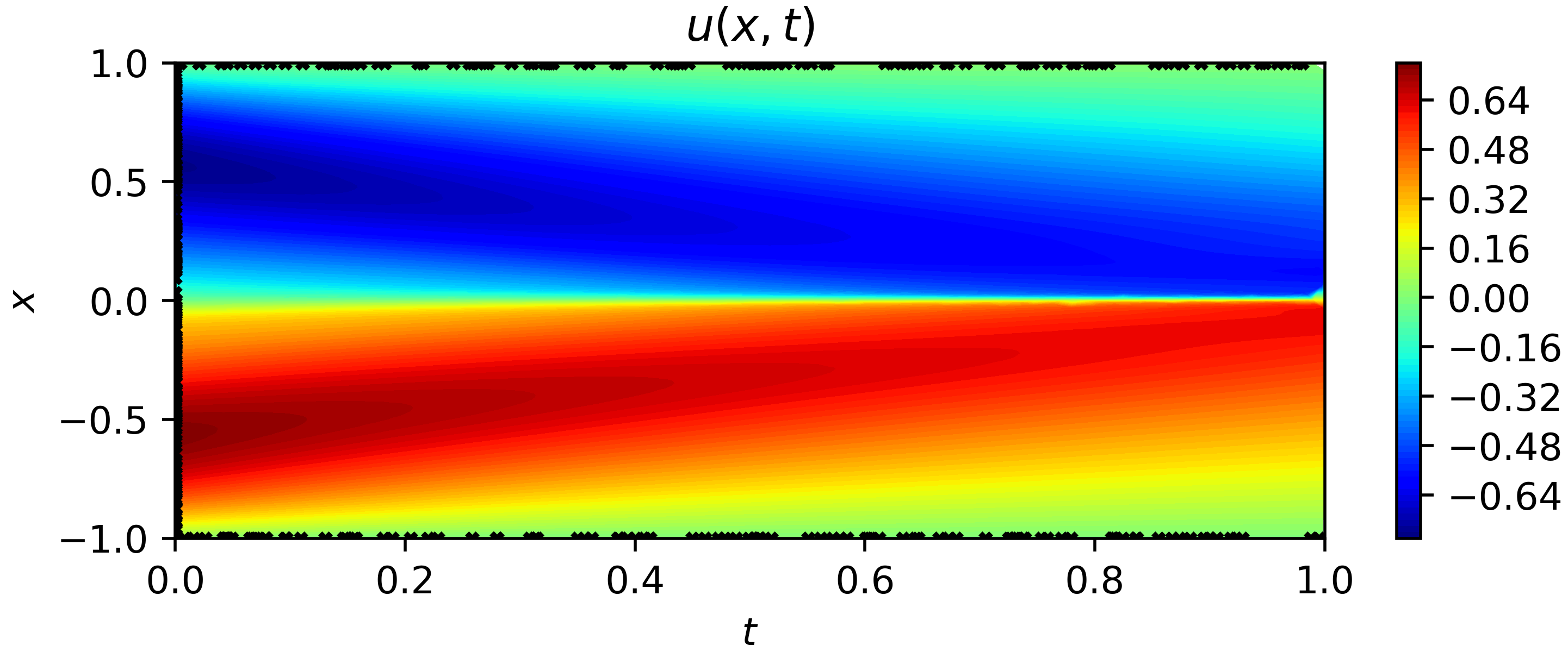
The result is shown as follows:

Use TensorBoard

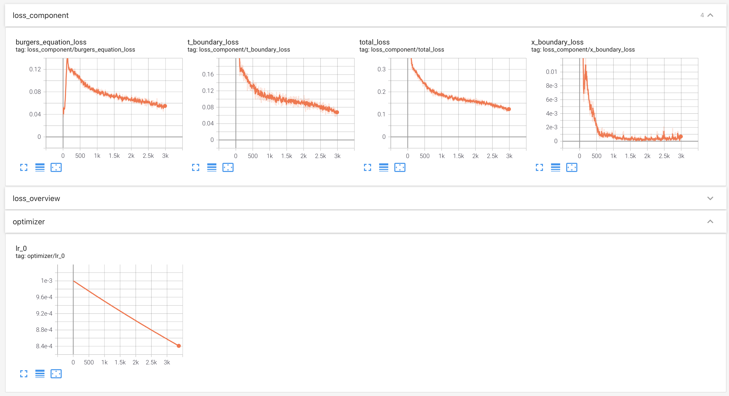
To monitor the training process, we employ TensorBoard. The learning rate, losses on different domains, and the total loss will be recorded automatically. Users can call Solver.summary_receiver() to get the instance of SummaryWriter. As default, one starts TensorBoard at ./network_idr:

tensorboard --logdir ./network_dir

Users can monitor the status of training:

See examples/burgers_equation.