forked from p94628173/idrlnet
42 lines
1.4 KiB
Markdown
42 lines
1.4 KiB
Markdown
# Volterra Integral Differential Equation
|
||
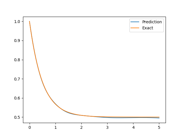
We consider the first-order Volterra type integro-differential equation on $[0, 5]$ (from [Lu et al. 2021](https://epubs.siam.org/doi/abs/10.1137/19M1274067)):
|
||
|
||
$$
|
||
\frac{d y}{d x}+y(x)=\int_{0}^{x} e^{t-x} y(t) d t, \quad y(0)=1
|
||
$$
|
||
with the ground truth $u=\exp(-x) \cosh x$.
|
||
|
||
## 1D integral with Variable Limits
|
||
The LHS is represented by
|
||
|
||
```python
|
||
exp_lhs = sc.ExpressionNode(expression=f.diff(x) + f, name='lhs')
|
||
```
|
||
|
||
The RHS has an integral with variable limits. Therefore, we introduce the class `Int1DNode`:
|
||
|
||
```python
|
||
fs = sp.Symbol('fs')
|
||
exp_rhs = sc.Int1DNode(expression=sp.exp(s - x) * fs, var=s, lb=0, ub=x, expression_name='rhs',
|
||
funs={'fs': {'eval': netnode,
|
||
'input_map': {'x': 's'},
|
||
'output_map': {'f': 'fs'}}},
|
||
degree=10)
|
||
```
|
||
We map `f` and `x` to `fs` and `s` in the integral, respectively.
|
||
The numerical integration is approximated by Gauss–Legendre quadrature with `degree=10`.
|
||
The difference between the RHS and the LHS is presented by a `pde_op.opterator.Difference` node,
|
||
|
||
```python
|
||
diff = sc.Difference(T='lhs', S='rhs', dim=1, time=False)
|
||
```
|
||
|
||
which generates a node with
|
||
- `input=(lhs,rhs)`;
|
||
- `output=(difference_lhs_rhs,)`.
|
||
|
||
The final result is shown as follows:
|
||
|
||
|
||
|
||
See `examples/Volterra_IDE`. |